


The coast is clear
Why analysing the data when a race driver is neither on the throttle nor the brakes is an excellent way of honing outright performance
BY CLAUDE ROUELLE
Download the original PDF from RaceCar Design Magazine!
In the last few articles, we have covered how to analyse the aspects of the braking part of a corner by looking at braking aggression, brake application point, and braking stability.
However, braking is only one small fraction of what can be analysed in a corner. Corner apex and exit speed can prove to be just as important, as it will define how much quicker a driver is through the corner and along the next straight.
To determine how well a driver can accelerate out of a corner, we can analyse how much time they are spending with no throttle or braking input through a given turn.
The time, or the percentage of the lap time spent neither on the brake nor the throttle, known as the coast factor, can in turn be used to determine how well a driver is performing relative to their competitors, and thus how a different driving style can be used to help them beat the competition.
For most corners, one of the fastest ways to take them is to minimise the time with no throttle or brake input. Table 1 shows the equations used in MoTeC i2 Pro to calculate the coast factor. The coast factor can be calculated as a Boolean function, meaning that when there is only a residual braking or throttle signal, the function will return a value of 1. The residual value of coasting should be determined when calibrating the throttle position sensor and the brake pressure sensor. We will integrate the time that the car is in the state of no inputs for each corner of the course to generate the coast KPI (key performance indicator) in a corner.
We can also track the total time coasting each lap by adding the corner times.
Table 1: Motec i2 coast factor math channels
| Name | Equation |
| Coast factor | choose(‘Throttle’ [%]<0.5 and ‘Brake’ [%]<0.5, 1, 0) |
| Coast factor corner KPI | integrate(‘Coast Factor’,’Corr Speed’ [km/h]>0,range_change(“Outings:Laps:Track Sections:Default:Straights”)) |
| Coast factor lap KPI | integrate(‘Coast Factor’,’Corr Speed’ [km/h]>0,range_change(“Outings:Laps”)) |
For this analysis, we will compare two NASCAR Truck drivers on
their qualifying laps at the Pocono Raceway tri-oval. Given that the two drivers were driving for peak performance, the variation in coast factor can be correlated to the lap time each driver achieved. This can, in turn, provide feedback to the driver on how to approach the track.
The coast factor can also be used in combination with other KPIs to
help provide information that can be utilised to determine set-up changes to make to a vehicle to minimise the coast factor magnitude.
NASCAR Truck in action at Pocono Raceway. Evaluating how long a driver coasts throughout a lap is a useful performance indicator

We will start by looking at the coast factor on a map to gauge where and how much the driver is coasting. Each loop shown is a different driver’s best lap. Red on the plot denotes where the drivers were coasting, while the plot is green when they were not. In the example shown in Figure 1, we can see that the black driver (denoted by the red surfaces on the inner loop) was coasting a significantly larger amount in the first and third corners when compared to the red driver. However, without additional knowledge of the driving style and without a lap time comparison, we cannot yet come to a conclusion over which driver was slower.
Figure 1: Coast factors for two NASCAR Truck drivers on their qualifying laps at Pocono
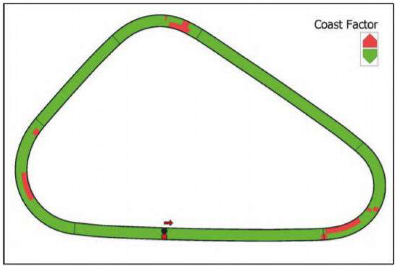
For most corners, one of the fastest ways for a driver to take them is to minimise the time with no throttle or brake input
To make a more informed conclusion, we can look at the minimum speed of the drivers using a second track plot. The minimum speed is defined as the lowest speed that the vehicle reaches during a corner. This can have a significant effect on which driver is quicker, especially on a track with a high concentration of straights, which is the case at Pocono Raceway.
Figure 2: Track map showing the speed of the black and red drivers on their best lap
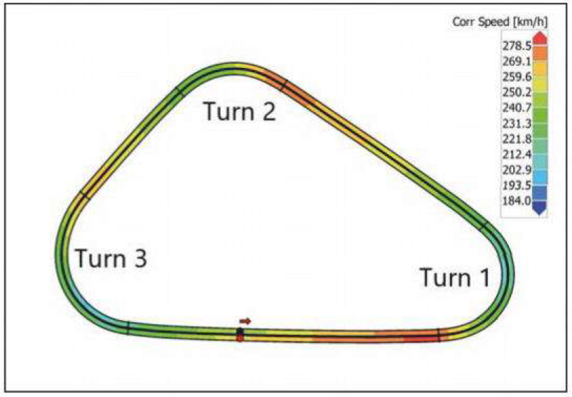
In Figure 2, a higher concentration of red denotes a higher speed while a higher concentration of blue correlates to a lower speed. The inner loop with the black dot refers to the black driver, while the outer loop with the red dot refers to the red driver.
In this plot, we can see that the black driver reduced speed much more significantly than the red driver in turn three, which in turn led to a lower end speed on the longest straight of the track. This gap becomes clearer in a speed trace and lap time variance comparison, which is shown in Figure 3.
Figure 3: Speed traces of our drivers, also showing the difference. Note the speed that the red driver carries on to the main straight
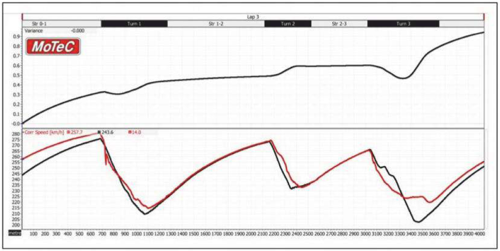
When the variance increases, it means that the red driver is increasing the gap to the black driver, and a negative slope means that the black driver is gaining on the red driver. Looking at the speed trace, we see that the biggest gains made by the red driver came as a result of a better performance in the third turn, as seen on the speed map.
This can be seen in the combination of the gap at the start of the lap from 0m to 600m and at the end of the lap from 3600m to 4000m.
This shows that while coasting through Turn 1 did not make a significant difference between the two drivers, in the third turn, coasting made a significant difference in driver performance. Based on the comparison of the two data traces of the laps, the driver with the black trace now has the knowledge to help gain ground during the race and be more competitive. Alternatively, the black driver’s team can also use the information learned from the session to modify the setup of the vehicle to better suit the driver’s style.
The analysis of performance can be extended to the full session as well. By looking at the percentage of time that each driver was spending coasting, we can have a strong understanding of the time delta between the two drivers as the race progresses. Figure 4 shows the lap time of the two drivers relative to the amount of time that each driver spent coasting.
Figure 4: This shows the lap times relative to the time each driver spends coasting
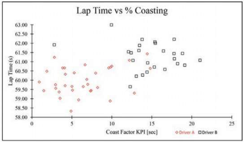
In this plot, we can see that there is a very gradual black driver lap time increase as a result of a higher amount of coasting. However, we can also see that there is a range of as much as two seconds between the fastest and slowest laps at the same coast factor. This is occurring as we are not considering other aspects of the course, such as traffic, tyre wear, or driver error. While the coast factor can indicate the level of performance of the driver during the race, it is important to consider the outside context when predicting driver performance.
In addition to its use as a single lap analysis tool, coasting can also be an effective technique for driving fast, but doing so in an efficient manner, which allows a driver to reach low fuel consumption goals.
By lifting and coasting, the driver can save fuel, allowing for a longer stint, which could make a difference to the number of pit stops required.
While there will still be circumstances in the driver's performance that could inherently induce a greater amount of coasting through a session, by lifting entirely, the driver will be saving fuel, which can have a direct effect on how far that driver can run in a stint.
To visualise how the drivers compared during the final fuel run of a race, we will compare the coast factor KPI during the complete lap to the level of fuel being saved. We can approximate the fuel saving by measuring the time during which the fuel flow of the vehicle is at its minimum.
Note that in some racing series, fuel flow sensors are forbidden during race weekends, but not necessarily during private practices. In contrast, some racing series require a car to have a fuel flow sensor so as to be able to hold the racecars to a maximum energy consumption.
Therefore, it is important to check the regulations and have predictions ready depending on the circumstances of the event.
It is also important to consider the outside context when predicting the driver performance
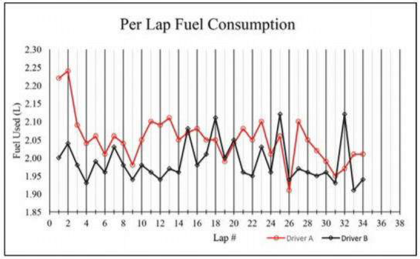
To begin with, we will look at the amount of fuel that the two drivers were using per lap during the event. When considering the fuel consumption, it is important to watch how the fuel consumption of two drivers could impact their final gap at the end of a race. If a driver can make one fewer pit stop, then they will have a significant
advantage over their competitor, which could be the difference between winning or losing a race.
In Figure 5, we can see that the amount of fuel that was consumed by the black driver was regularly lower than the amount of fuel that was consumed by the red driver during the 37-lap stint. This will mean that the red driver, despite the greater pace that can be seen in their fastest laps in Figure 4, will have to pit earlier than the black driver. In the case that this was intended to be the final stint, this would mean that the red driver would be pulled out of contention due to overconsumption.
Therefore, it can be imperative to track the fuel-saving measures like coast factor to make sure that the driver is doing all that they can to maintain pace without sacrificing lap time excessively.
Figure 5: The fuel consumption for each lap. The black driver is usually using less fuel
To determine the correlation between the coast factor and the amount of fuel saved, we will plot the amount of time with minimal fuel flow, the fuel savings on the y-axis, and the coast factor on the x-axis, to determine the correlation the two variables have to each other.
The goal with this plot is to track how much fuel is being saved just by coasting during the lap versus the amount being saved when off the throttle during braking.
Figure 6 plots the black and red drivers' coast factors and fuel savings for each lap in a stint. Note that there is a strong correlation between the amount of time that is spent coasting and the amount of fuel saved, with the black driver saving more than the red. We can also see that there is about six seconds of constant fuel savings as a result of just braking during a corner. This can be correlated back to the fuel flow and can be used to determine the worst-case fuel economy for a lap, which can, in turn, be used for determining fuel cell sizing for a weekend (if this is allowed).
Figure 6: The correlation of coast factor to the fuel savings for each lap during a stint
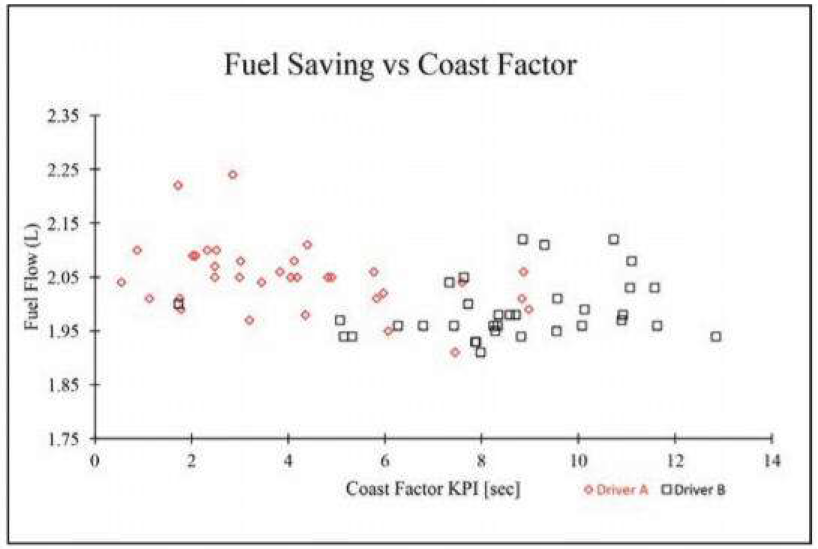
Table 2: Motec i2 fuel flow math channels
| Name | Equation |
| Fuel flow | derivative(‘Fuel Level’ [l]) |
| Fuel saving | choose(‘Fuel Flow’>-0.01,1,0) |
| Fuel saving KPI | integrate(‘Fuel Saving’,1,range_change(“Outings:Laps”)) |
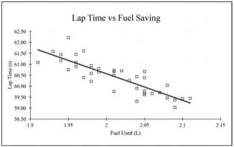
The last element of fuel saving that can be tracked using the coast factor is the lap time the driver was able to perform versus the amount of fuel that was consumed. This can be especially useful when working on a racecar without telemetry, as it can allow a race strategist to predict the lap time required to achieve a given stint length. While there will be noise in the data, this can still be the best estimate and will allow a strategist to advise the lap time goals for a driver to hit.
Figure 7 shows the lap time that would be required for the driver to save a given amount of fuel. In this case, we see that the driver could save about 0.05 litres for every second slower they drive. This can, in turn, be used by a race strategist to plan when a driver starts to save fuel or whether the gains from coasting are worth it. This will vary for different conditions and for different courses, but it can be a strong asset to gauge when to pit and how aggressively a race driver can drive during a given fuel run.
All of this can be learned from how much the driver is coasting.
Figure 7: Comparison of lap time vs fuel used. This is very useful for devising strategies
In conclusion, coasting is a non-trivial technique that can be a balance between high performance and efficient driving. It can be a tool used by the race engineer to describe the intermediate area of
a corner and show the cause of a higher corner exit speed. On the driver’s side, it can be used as a strategy tool to gain an advantage over a competitor, either in the pits or in overtaking. By having the driver practice coasting, the race strategist can then predict time targets that the driver should be hitting to conserve fuel during an event.
When looking at the coast factor, the complexities of a vehicle become ever apparent, and the gains from even the smallest of areas can become ever more present.


